As a part of a University level GIS course I taught I needed to generate some raster data for a lab exercise on map algebra. I wrote a function to “rasterize” polyline data I had on hand, that is, to convert the discrete polyline data to a continuous density surface. This type of operation used in things like land use regression models or in metrics of walkability or bikeability, which require all input data to be continuous surfaces. Here I develop a function to automate the process of creating such a surface in R using sf, raster and tidyverse packages.
rasterize_lines(input_study_area,input_linestring,cell_size=100,buffer_width=300,mask=F)
Arguments
- input_study_area:
sfpolygon or multipolygon - input_linestring:
sflinestring or multilinestring - cell_size: Desired spatial resolution of the output raster (i.e. in metres)
- buffer_width: Buffer length from which to calculate line densities from each raster cell centroid.
- mask: If
TRUEthen the output raster is clipped by the study area boundary. IfFALSEthen the output raster extent is equal to bounding box of study area boundary
Value
An RasterLayer file
Explanation
The function rasterize_lines takes the following steps to rasterize the polylines:
- Create empty raster surface of specified grid cell size and study area extent
- Generate buffers of specified length from the centroid of the empty raster surface
- Split the polylines by the centroid buffers layer
- Sum the length of polylines within each buffer in the centroid buffers layer
- Assign the length within each buffer to the associated raster
- Output raster where each grid cell has the value of the length of the polylines within the specified buffer length of the cell centroid
The function is defined below:
rasterize_lines <- function(input_study_area,input_linestring,cell_size=100,buffer_width=300,mask=F){
  require(sf)
  require(raster)
  require(tidyverse)

  if(st_crs(input_study_area)$proj4string==st_crs(input_linestring)$proj4string){ #check that both study area and polyline files are in the same coordinate system and projection


    print("Generating grid...")
    #Create template raster from Study Area extent (empty raster with the extent of the study area, and cell size as indicated)
    raster_template <- raster(extent(input_study_area), resolution = cell_size,
                              crs = st_crs(input_study_area)$proj4string)
    print("Buffering grid cell centroids....")

    rast_point <- rasterToPoints(raster_template, spatial = TRUE) %>%
      st_as_sf() #create point layer from template raster based on the centroid

    rast_point_buff <- st_buffer(rast_point,dist=buffer_width)#create buffers from raster cell centroids of specified width


    print("Finding intersections between grid cell centroid buffers and input lines...")

    #find intersection points between buffer boundaries and input_linestring (e.g. isolate buffers that actually intersect with polyline data)
    rast_point_buff_ls <- st_cast(rast_point_buff,"LINESTRING")

    input_linestring <- st_geometry(input_linestring) %>%
      st_transform(crs = st_crs(rast_point_buff_ls)$proj4string)#reduce size of dataset and ensure proj4strings are the same

    int_points <- st_intersection(rast_point_buff_ls,input_linestring) %>% #find intersection of road lines and centroid buffers
      st_cast("MULTIPOINT") %>%
      st_cast("POINT")

    print("Splitting input lines by intersections...")

    int_points_buff <- st_buffer(int_points,dist = 0.0000001) %>% st_combine() #buffer points to very small distance

    grid <- st_make_grid(rast_point_buff,what = "polygons",n = c(10,10))#split bounding box of polygon into grid
    grid <- grid[st_intersects(grid,int_points_buff,sparse = F)[,1]]#remove grid cells that do not intersect with the roads
    printPercent <- seq(from = 0, to = length(grid),by=(length(grid)/20))

    #iterate through each grid cell and intersect roads with grid cell, split the line geometry within that cell by the intersection buffers
    for (i in 1:length(grid)) {
      temp <- st_intersection(int_points_buff, grid[i])
      input_linestring <- st_difference(input_linestring, temp)

      if (i %in% round(printPercent)) {
        print(paste(round(i / length(grid) * 100, 0),
                    "% of lines split"))
      }
    }

    print("Calculating lengths of split polylines...")

    input_linestring_ls <- input_linestring %>%
      st_cast("MULTILINESTRING") %>%
      st_cast("LINESTRING")#convert to linestring to isolate non-contiguous lines

    input_linestring_ls <-
      st_sf(data.frame(length_m = st_length(input_linestring_ls)), geometry = input_linestring_ls) #calculate each line segment length

    print("Spatially aggregating road lengths by each cell centroid buffer")

    #Join to line polygons, sum line segment length within each polygon
    rast_point_buff <-
      st_sf(data.frame(ID = seq(1, length(st_geometry(rast_point_buff))),
                       geometry = rast_point_buff)) #create sf object with the geometry of the point buffer

    rast_point_buff <- rast_point_buff %>%
      st_join(input_linestring_ls) %>% #join lines split by buffer geometry and associated lengths to the buffer it falls within (e.g. points buffer is the target layer, input lines are join layer)
      group_by(ID) %>%
      summarize(line_length = sum(length_m),`.groups`="drop_last") %>%
      mutate(line_length = replace_na(line_length, 0)) %>%
      st_set_agr(c(line_length = "identity", ID = "identity")) #specify attribute-geometry relationship to avoid warning since we already know line_length represents the value over the entire geometry

    rast_point_buff_cntrd <- st_centroid(rast_point_buff)

    output_rast = rasterize(rast_point_buff_cntrd,
                            raster_template,
                            field = "line_length",
                            fun = sum)

    if(mask==TRUE){

      output_rast <- mask(output_rast, as(input_study_area, "Spatial"))


    }


  }else{
    "Input study area must be in the same projection as input lines"


  }

    return(output_rast)

}
Example
I want to map the density of seperated bikelanes in Vancouver, BC as a continuous raster surface. I have two sf objects:
vancouver_boundaryseparated_bl
Lets take at the boundary data:
vancouver_boundary %>% structure()## Simple feature collection with 1 feature and 1 field
## geometry type: POLYGON
## dimension: XY
## bbox: xmin: 483690.9 ymin: 5449535 xmax: 498329.2 ymax: 5462381
## projected CRS: NAD83 / UTM zone 10N
## area geometry
## 1 116255573 [m^2] POLYGON ((491475.3 5450127,...ggplot(vancouver_boundary) +
geom_sf() +
theme_bw()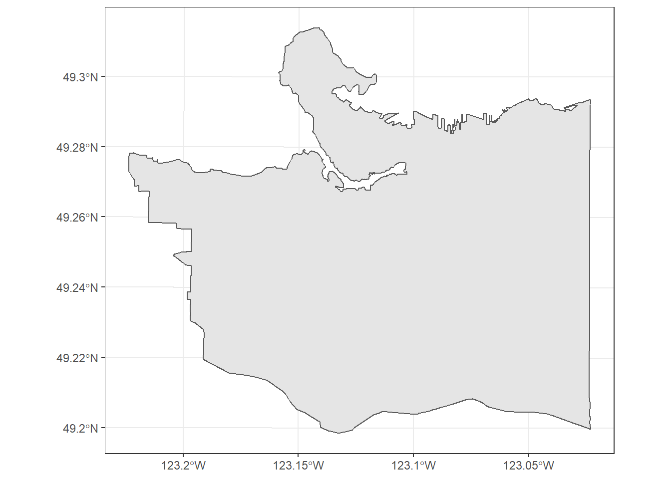
Lets take a look at the separated bikelane data:
separated_bl%>% structure()## Simple feature collection with 193 features and 9 fields
## geometry type: MULTILINESTRING
## dimension: XY
## bbox: xmin: 483723.4 ymin: 5449450 xmax: 498302.6 ymax: 5462403
## projected CRS: NAD83 / UTM zone 10N
## First 10 features:
## UNIQUE_ID ROUTE_NAM STREET_NAM TPL_TYPE STATUS
## 1 1 Burrard Brdg Burrard Bridge Protected Bike Lanes Active
## 2 5 Seaside Bypass W 2nd Ave Protected Bike Lanes Active
## 3 7 Knight St Bridge Knight St Bridge Protected Bike Lanes Active
## 4 9 Laurel Overpass Laurel Overpass Protected Bike Lanes Active
## 5 14 South Terminal L/S of Terminal Protected Bike Lanes Active
## 6 19 Central Velley E 1st Ave Protected Bike Lanes Active
## 7 20 Knigth St Bridge On Ramp Knight Bridge Protected Bike Lanes Active
## 8 24 Cornwall Cornwall Protected Bike Lanes Active
## 9 27 Pacific Pacific St Protected Bike Lanes Active
## 10 28 Kerr St Kerr St Protected Bike Lanes Active
## LENGTH YEAR_CONST DIRECTION STREET_TYP geometry
## 1 1059 1990 NS Arterial MULTILINESTRING ((490372 54...
## 2 146 2009 NS Arterial MULTILINESTRING ((491661.8 ...
## 3 741 1990 NS Arterial MULTILINESTRING ((494374.9 ...
## 4 177 0 NS Residential MULTILINESTRING ((490971.9 ...
## 5 1061 2003 EW Lane MULTILINESTRING ((492866.9 ...
## 6 148 0 EW Residential MULTILINESTRING ((492538.4 ...
## 7 184 2003 NS Arterial MULTILINESTRING ((494251.7 ...
## 8 182 1990 NS Arterial MULTILINESTRING ((489421.9 ...
## 9 311 2016 EW Arterial MULTILINESTRING ((490225.5 ...
## 10 143 2009 NS Arterial MULTILINESTRING ((496922.1 ...ggplot(separated_bl) +
geom_sf() +
theme_bw()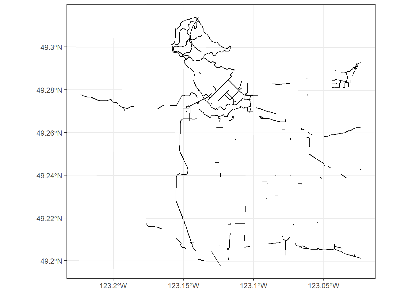
Note that both sf objects have the same coordinate reference system (CRS). This function needs each sf object to be in the same projected coordinate system.
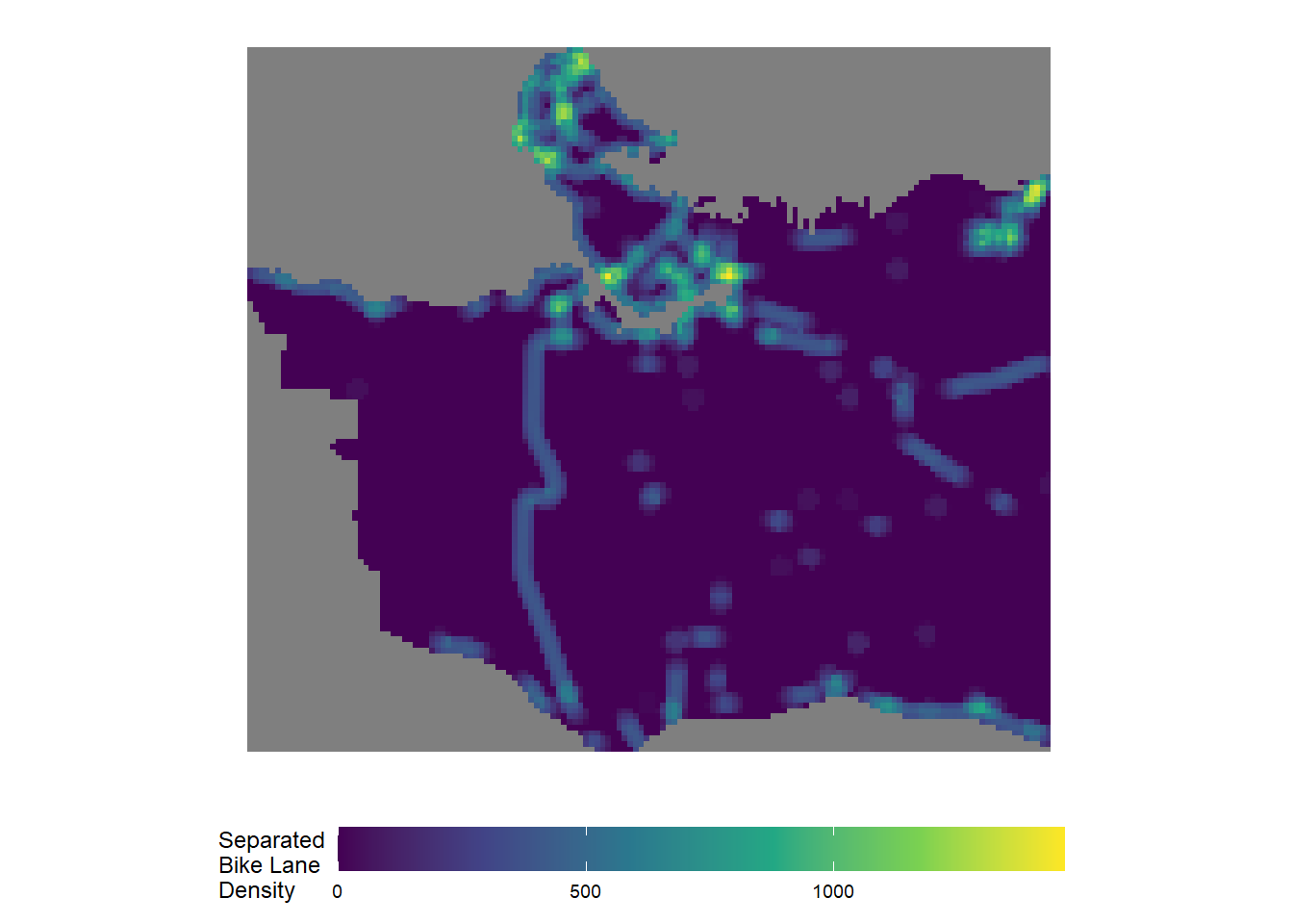
Now I input the parameters into the rasterize_lines() function. I chose a 100m by 100m cell size, and want to calculate the density of separated bikelanes within 300m of the centroid of each cell (500m buffer):
sep_bl_rast <- rasterize_lines(input_study_area = vancouver_boundary,
                                          input_linestring = separated_bl,
                                          cell_size = 100,
                                          buffer_width = 200,
                                          mask=TRUE)
## [1] "Generating grid..."
## [1] "Buffering grid cell centroids...."
## [1] "Finding intersections between grid cell centroid buffers and input lines..."
## [1] "Splitting input lines by intersections..."
## [1] "5 % of lines split"
## [1] "11 % of lines split"
## [1] "15 % of lines split"
## [1] "20 % of lines split"
## [1] "25 % of lines split"
## [1] "29 % of lines split"
## [1] "35 % of lines split"
## [1] "40 % of lines split"
## [1] "45 % of lines split"
## [1] "51 % of lines split"
## [1] "55 % of lines split"
## [1] "60 % of lines split"
## [1] "65 % of lines split"
## [1] "69 % of lines split"
## [1] "75 % of lines split"
## [1] "80 % of lines split"
## [1] "85 % of lines split"
## [1] "91 % of lines split"
## [1] "95 % of lines split"
## [1] "100 % of lines split"
## [1] "Calculating lengths of split polylines..."
## [1] "Spatially aggregating road lengths by each cell centroid buffer"Once the function runs the output is a RasterLayer file. We can enable mapping in ggplot by converting it to a data.frame:
sep_bl_rast_df <- as.data.frame(sep_bl_rast, xy = TRUE)#covert raster file to dataframe to enable mapping in ggplotggplot() +
geom_raster(data = sep_bl_rast_df,aes(x=x,y=y,fill=layer)) +
scale_fill_viridis_c(name = "Separated\nBike Lane\nDensity") +
xlab("Longitude") +
ylab("Latitude") +
coord_equal() +
theme_map() +
theme(legend.position="bottom") +
theme(legend.key.width=unit(2, "cm"))