To produce kernel density estimates (KDE) of point processes in a linear network:
\[\lambda(z)= \sum_{i=1}^{n} \frac{1}{\tau} k(\frac{d_{iz}}{\tau})y_i\]
Using the Quartic function:
\[\lambda(z)= \sum_{i=1}^{n} \frac{1}{\tau}(\frac{3}{\pi}(1-\frac{d_{iz}^2}{\tau^2}))y_i\]
Where,
\(\lambda\)(z) = density at location z;
\(\tau\) is bandwidth linear network distance;
\(k\) is the kernel function, typically a function of the ratio of \(d_{iz}\) to \(\tau\);
\(d_{iz}\) is the linear network distance from event \(i\) to location \(z\).
I wanted to implement a network-based KDE in R based on the algorithm outlined in Xie & Yan (2008). The network KDE is a a 1-D version of the planar kernel density estimator, with \(\tau\) (bandwidth) based on network distances, rather than Euclidean distances and the output is based on lixels, a 1-D version of pixels), rather than pixels across 2-D euclidean space.
In this post I use data from Vancouver, BC as a case study for implementing a network kernel density estimator of points in a network in R.
Set Up
library(tidygraph)
library(igraph)
library(stplanr)
library(cancensus)
library(osmdata)
library(dplyr)
library(sf)
library(ggplot2)
library(stringr)
Getting the example data
The first step is to load example data.
Study Area Extent
I use the get_census function from the cancensus package to extract a sf object with POLYGON geometries, representing the study extent: the City of Vancouver.
study_area <- get_census(dataset='CA16', regions=list(CSD="5915"),
                     level='CSD', use_cache = FALSE,geo_format = "sf") %>%
  filter(name=="Vancouver (CY)") %>%
  st_transform(crs = 26910)
##
Downloading: 7.6 kB
Downloading: 7.6 kB
Downloading: 7.6 kB
Downloading: 7.6 kB
Downloading: 24 kB
Downloading: 24 kB
Downloading: 40 kB
Downloading: 40 kB
Downloading: 40 kB
Downloading: 40 kB
Downloading: 52 kB
Downloading: 52 kB
Downloading: 52 kB
Downloading: 52 kBggplot(study_area) +
geom_sf() +
coord_sf() +
theme_void()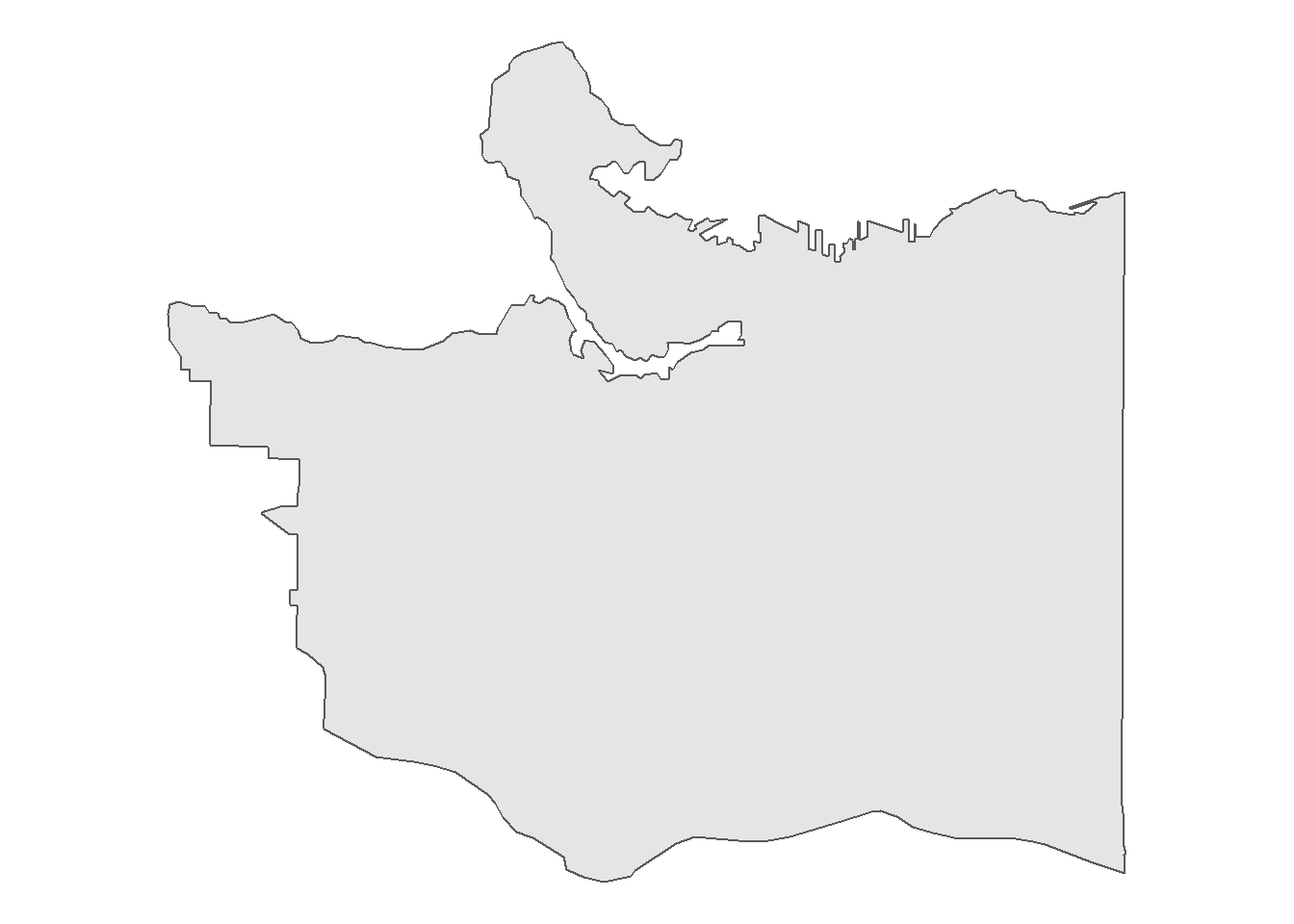
Road Network Data
Next I use the osmdata package to download street network files for the City of Vancouver. The getbb() function defines a bounding box for the City of Vancouver.
bbx <- getbb("Vancouver, BC")Next we use the opq() and add_osm_feature functions to obtain open street map road network data. The osmdata_sf()
streets <- bbx %>%
  opq()%>%
  add_osm_feature(key = "highway",
                  value=c("residential", "living_street",
                            "service","unclassified",
                            "pedestrian", "footway",
                            "track","path","motorway", "trunk",
                          "primary","secondary",
                          "tertiary","motorway_link",
                          "trunk_link","primary_link",
                          "secondary_link",
                          "tertiary_link")) %>%
  osmdata_sf()


streets_sf <- st_transform(streets$osm_lines,crs=26910) %>%
  filter(st_intersects(.,study_area,sparse=FALSE))

ggplot() +
  geom_sf(data = streets_sf,
          aes(color=highway),
          size = .4,
          alpha = .65)+
  theme_void()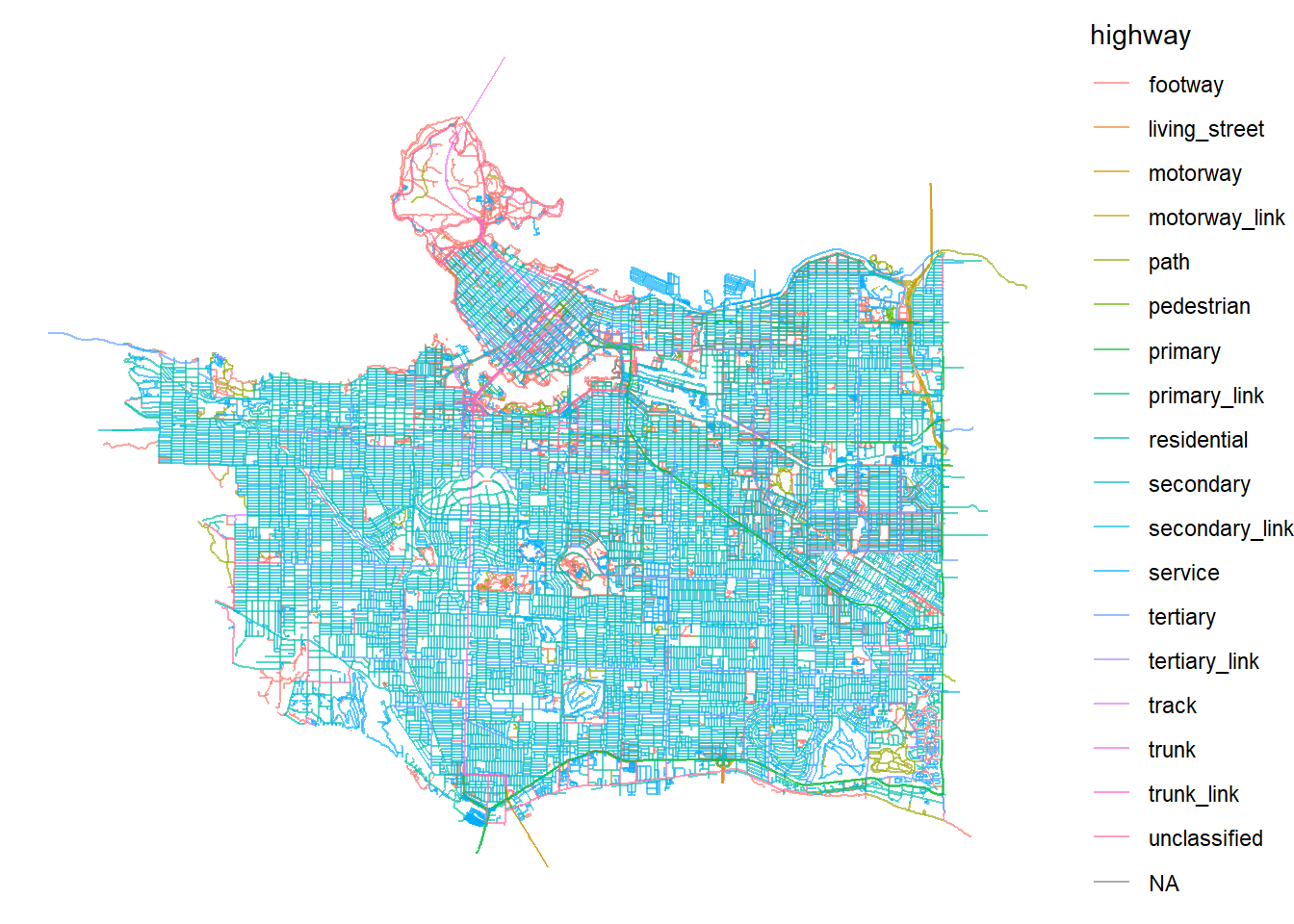
Police Report Data
Finally I get point data of police reports in Vancouver from the City of Vancouver. I subset the data to only include vehicle collisions reported to police in 2018 (last full year of data available).
url <- "ftp://webftp.vancouver.ca/opendata/csv/crime_csv_all_years.zip"
temp <- tempfile()
download.file(url, temp)
crime <- read.csv(unz(temp, "crime_csv_all_years.csv"))
unlink(temp)

collisions <- crime %>%
  filter(YEAR==2018 & str_detect(TYPE,"Vehicle Collision"))%>%
  st_as_sf(.,coords = c("X","Y"),crs=26910)
Locations of police reported vehicle collisions are below.
ggplot(collisions) +
  geom_sf() +
  coord_sf() +
  theme_void()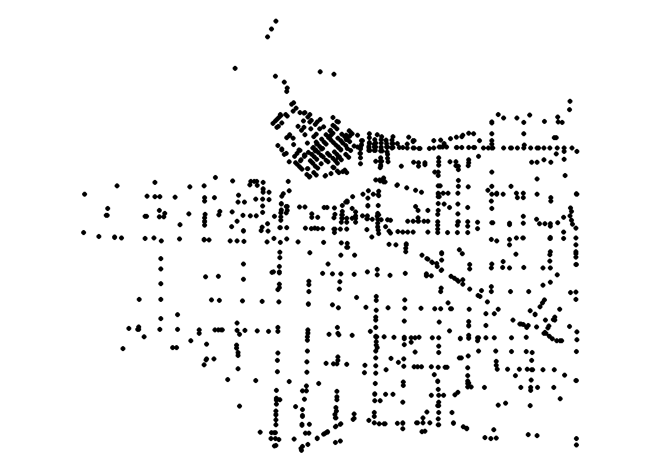
Now we have the data we need to try and estimate the density of police-reported collisions or “hotspots” in the City of Vancouver.
NOTE: These data do not differentiate between different types of collisions between road users, and police road collision data consistently miss out on the majority of crashes that occur to active transport users (bicyclists and pedestrians).
Prepare the network data
In the algorithm outlined in Xie & Yan (2008) the resulting density estimates on a network are based on a spatial unit of analysis they term a lixel. Lixels are basically the 1-D version of a pixel, and refer to how long the segments in our network are from which we calculate densities of events.
To create a lixelized network I combine the split_lines() and the lixelize network() functions.
The split_lines() function has three arguments:
- input_lines:
sfobject withLINSETRINGorMULTILINESTRINGgeometry - max_length: the lixel size, defined by the maximum length of an individual linestring in the data.
- id: a unique id for each line segment in the
sfobject
The split_lines() function is given below:
split_lines <- function(input_lines, max_length, id) {

  input_lines <- input_lines %>% ungroup()

  geom_column <- attr(input_lines, "sf_column")

  input_crs <- sf::st_crs(input_lines)

  input_lines[["geom_len"]] <- sf::st_length(input_lines[[geom_column]])

  attr(input_lines[["geom_len"]], "units") <- NULL
  input_lines[["geom_len"]] <- as.numeric(input_lines[["geom_len"]])

  too_short <- filter(select(all_of(input_lines),all_of(id), all_of(geom_column), geom_len), geom_len < max_length) %>% select(-geom_len)

  too_long <- filter(select(all_of(input_lines),all_of(id), all_of(geom_column), geom_len), geom_len >= max_length)

  rm(input_lines) # just to control memory usage in case this is big.

  too_long <- mutate(too_long,
                     pieces = ceiling(geom_len / max_length),
                     fID = 1:nrow(too_long)) %>%
    select(-geom_len)

  split_points <- sf::st_set_geometry(too_long, NULL)[rep(seq_len(nrow(too_long)), too_long[["pieces"]]),] %>%
    select(-pieces)

  split_points <- mutate(split_points, split_fID = row.names(split_points)) %>%
    group_by(fID) %>%
    mutate(piece = 1:n()) %>%
    mutate(start = (piece - 1) / n(),
           end = piece / n()) %>%
    ungroup()

  new_line <- function(i, f, t) {
    lwgeom::st_linesubstring(x = too_long[[geom_column]][i], from = f, to = t)[[1]]
  }

  split_lines <- apply(split_points[c("fID", "start", "end")], 1,
                       function(x) new_line(i = x[["fID"]], f = x[["start"]], t = x[["end"]]))

  rm(too_long)

  split_lines <- st_sf(split_points[c(id)], geometry = st_sfc(split_lines, crs = input_crs))

  lixel <- rbind(split_lines,too_short) %>% mutate(LIXID = row_number())

  return(lixel)
}
The second function needed to prepare the network data is the lixelize_network function. This takes two arguments, an sf object with LINESTRING or MULTILINESTRING geometry and the lixel_length argument. This function will create two lixelized networks: 1) the output network where the line data are lixelized and no segment is larger than the a given pixel size and 2) a shortest distance network which will be used to calculate road network lengths in our network kernel density estimates that we will dive into shortly.
The lixelize network function is given below:
lixelize_network <- function(sf_network,max_lixel_length,uid){
  print("Splitting input spatial lines by lixel length...")
  target_lixel <- split_lines(input_lines = sf_network,max_length = max_lixel_length,id = uid)
  print("Create corresponding shortest distance network...")
  shortest_distance_network <- split_lines(input_lines = target_lixel,max_length = max_lixel_length/2,id = uid)
  return(list(target_lixel=target_lixel,shortest_distance_network=shortest_distance_network))
}
Our approach varies from Xie and Yan (2008) in that we define a “maximum” length for lixels based on the split_lines() function, and segments that are larger than the specified length are split into equal sized lixels. Instead of having \(n\) lixels with 1 extra “residual lixel” we instead have \(n\)+1 lixels of equal length, under the lixel limit. For example a 45m segment with a maximum lixel length of 10m would be split into 5 segments of 9m instead of 4 lixels of 10m and a residual lixel of 5m.
Before we use the functions described above to create a network of basic linear units under a maximum length (e.g. lixelized network), we will clean our existing osm data by removing unconnected segments of roads using the stplanr.
First we convert our sf road network to a spatial lines network object using the SpatialLinesNetwork() function, then clean use the sln_clean_graph() function to keep the largest set of connected road segments within our dataset.
network_sln <- SpatialLinesNetwork(streets_sf)## Warning in SpatialLinesNetwork.sf(streets_sf): Graph composed of multiple
## subgraphs, consider cleaning it with sln_clean_graph().network_sln <- sln_clean_graph(network_sln)# Remove unconnected roads## Input sln composed of 8750 graphs. Selecting the largest.ggplot(network_sln@sl) +
geom_sf() +
coord_sf() +
theme_void()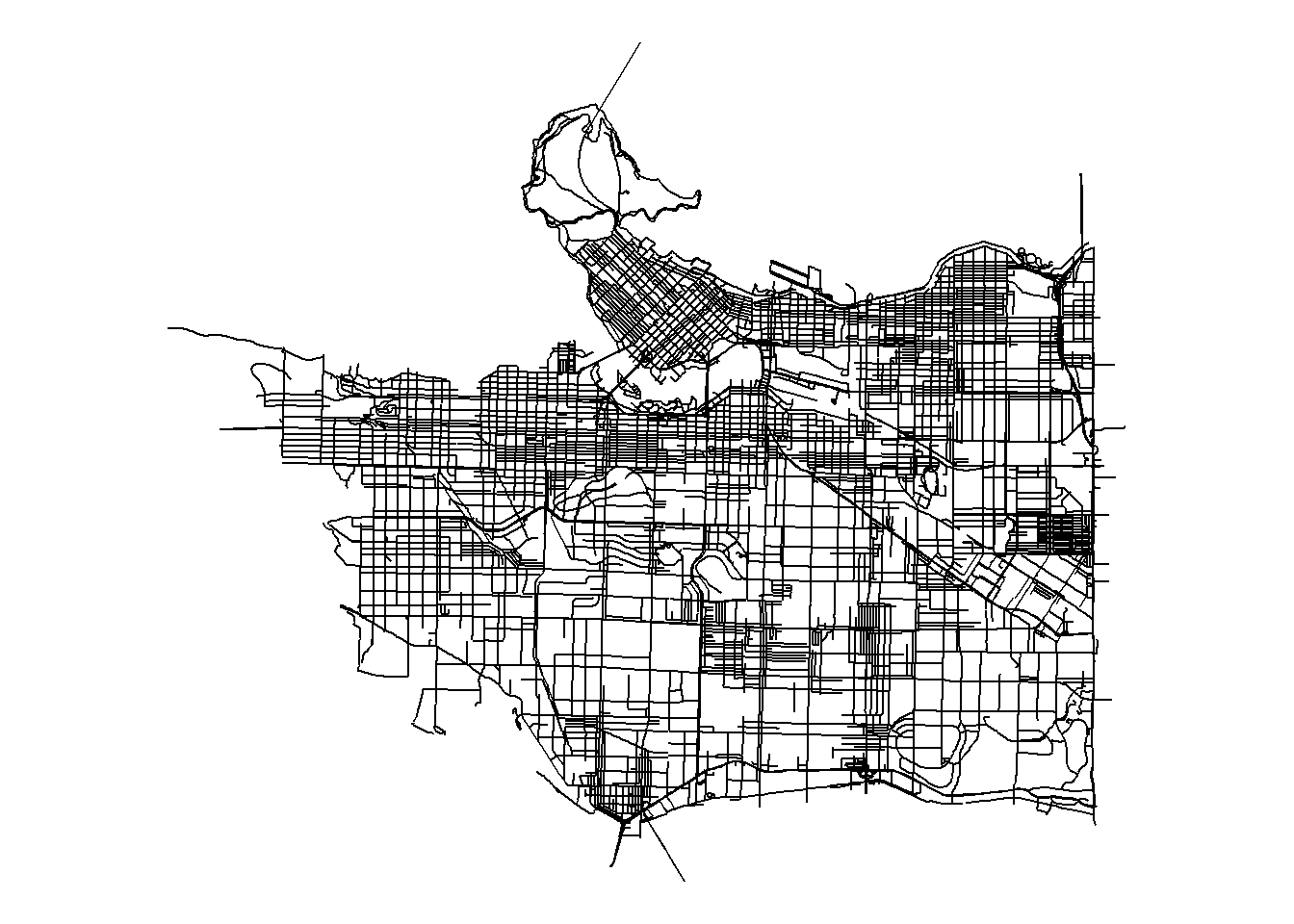
Check out the following link for more on the stplanr package https://cran.r-project.org/web/packages/stplanr/vignettes/stplanr-paper.html. For now we are only using the one function from the package to clean our network.
Lixelize the cleaned network
Next step is to lixelize the cleaned network. I choose a 25m maximum lixel length (e.g. every linear segment in the network will be 25m or under. This function may take some time to run.
lixel_list_25m <- lixelize_network(
  sf_network = network_sln@sl,
  max_lixel_length = 25,
  uid = "osm_id"

)
## [1] "Splitting input spatial lines by lixel length..."
## [1] "Create corresponding shortest distance network..."str(lixel_list_25m)## List of 2
## $ target_lixel :Classes 'sf' and 'data.frame': 60217 obs. of 3 variables:
## ..$ osm_id : chr [1:60217] "4231647" "4231647" "4231647" "4231647" ...
## ..$ geometry:sfc_LINESTRING of length 60217; first list element: 'XY' num [1:3, 1:2] 487784 487794 487807 5455047 5455043 ...
## ..$ LIXID : int [1:60217] 1 2 3 4 5 6 7 8 9 10 ...
## ..- attr(*, "sf_column")= chr "geometry"
## ..- attr(*, "agr")= Factor w/ 3 levels "constant","aggregate",..: NA NA
## .. ..- attr(*, "names")= chr [1:2] "osm_id" "LIXID"
## $ shortest_distance_network:Classes 'sf' and 'data.frame': 119970 obs. of 3 variables:
## ..$ osm_id : chr [1:119970] "4231647" "4231647" "4231647" "4231647" ...
## ..$ geometry:sfc_LINESTRING of length 119970; first list element: 'XY' num [1:3, 1:2] 487784 487794 487795 5455047 5455043 ...
## ..$ LIXID : int [1:119970] 1 2 3 4 5 6 7 8 9 10 ...
## ..- attr(*, "sf_column")= chr "geometry"
## ..- attr(*, "agr")= Factor w/ 3 levels "constant","aggregate",..: NA NA
## .. ..- attr(*, "names")= chr [1:2] "osm_id" "LIXID"The output is a list of two lixelized networks. The first is the lixelized network with the specified length, and the second is the same network but with lixel lengths half the size of indicated. This is the network that will be used in the network kernel density function to calculate shortest network distances from each lixel to each event on the network. More detail on that in the following section.
Prepare the point data
Here I need to ensure that the point data are lined up with the cleaned network data. I use a function called st_snap_points which “snaps” the points to the location of the nearest road segment within a specified distance tolerance. The function is given below:
st_snap_points = function(x, y, max_dist = 1000) {

  if (inherits(x, "sf")) n = nrow(x)
  if (inherits(x, "sfc")) n = length(x)

  out = do.call(c,
                lapply(seq(n), function(i) {
                  nrst = st_nearest_points(st_geometry(x)[i], y)
                  nrst_len = st_length(nrst)
                  nrst_mn = which.min(nrst_len)
                  if (as.vector(nrst_len[nrst_mn]) > max_dist) return(st_geometry(x)[i])
                  return(st_cast(nrst[nrst_mn], "POINT")[2])
                })
  )
  return(out)
}
We snap the points to our road network with a 20m tolerance:
coll_snp <- st_snap_points(collisions,network_sln@sl,max_dist = 20) #this only returns the geometry - doesn't preserve attributes

coll_snp <- st_sf(collisions %>%
                  st_drop_geometry() %>%
                  mutate(geom=coll_snp)) #rerturn the attributes to the snapped locations
Calculate Network Kernel Density
The function I have created here for calculating density of events on a network follows the algorithm outline in Xie and Yan (2008) and takes advantage of functionality from sf, igraph and tidygraph to to calculate shortest distances from each lixel in our network to the point processes we specify. Much of the code in this function is adapted from an excellent resource on using these packages for network analysis: https://www.r-spatial.org/r/2019/09/26/spatial-networks.html
The network_kde() function is defined below:
#function for calculating the centre of
st_line_midpoints <- function(sf_lines = NULL) {

  g <- st_geometry(sf_lines)

  g_mids <- lapply(g, function(x) {

    coords <- as.matrix(x)

    # this is just a copypaste of maptools:::getMidpoints()):
    get_mids <- function (coords) {
      dist <- sqrt((diff(coords[, 1])^2 + (diff(coords[, 2]))^2))
      dist_mid <- sum(dist)/2
      dist_cum <- c(0, cumsum(dist))
      end_index <- which(dist_cum > dist_mid)[1]
      start_index <- end_index - 1
      start <- coords[start_index, ]
      end <- coords[end_index, ]
      dist_remaining <- dist_mid - dist_cum[start_index]
      mid <- start + (end - start) * (dist_remaining/dist[start_index])
      return(mid)
    }

    mids <- st_point(get_mids(coords))
  })

  out <- st_sfc(g_mids, crs = st_crs(sf_lines))
  out <- st_sf(out)
  out <- bind_cols(out,sf_lines %>% st_drop_geometry()) %>% rename(geom=out)
}


network_kde <- function(lixel_list,point_process,bandwidth = 100,n_cores=1,attribute=1,point_process_is_lixel_midpoint=FALSE){


  #3. Create a network of lixels by establishing the network topology between lixels as well as between lixels and lxnodes.

  #Define topology for calculating shortest distances by converting lixel with half the length to calculate distances
  #The shorter the lixel length the more accurate the calculation of network distance from nearest node of source lixel to nearest node of target lixel
  print("Defining network topology...")

  require(parallel)
  require(doParallel)
  require(igraph)
  require(tidygraph)
  require(sf)
  require(dplyr)


  # Create nodes at the start and end point of each edge

  nodes <- lixel_list$shortest_distance_network %>%
    st_coordinates() %>%
    as_tibble() %>%
    rename(LIXID = L1) %>%
    group_by(LIXID) %>%
    slice(c(1, n())) %>%
    ungroup() %>%
    mutate(start_end = rep(c('start', 'end'), times = n()/2))

  # Give each node a unique index

  nodes <- nodes %>%
    mutate(xy = paste(.$X, .$Y),
           xy = factor(xy, levels = unique(xy))) %>%
    group_by(xy)%>%
    mutate(nodeID = cur_group_id()) %>%
    ungroup() %>%
    select(-xy)

  # Combine the node indices with the edges

  start_nodes <- nodes %>%
    filter(start_end == 'start') %>%
    pull(nodeID)

  end_nodes <- nodes %>%
    filter(start_end == 'end') %>%
    pull(nodeID)

  lixel_list$shortest_distance_network = lixel_list$shortest_distance_network %>%
    mutate(from = start_nodes, to = end_nodes)

  # Remove duplicate nodes
  nodes <- nodes %>%
    distinct(nodeID, .keep_all = TRUE) %>%
    select(-c(LIXID, start_end)) %>%
    st_as_sf(coords = c('X', 'Y')) %>%
    st_set_crs(st_crs(lixel_list$shortest_distance_network))

  # Convert to tbl_graph
  graph <- tbl_graph(nodes = nodes, edges = as_tibble(lixel_list$shortest_distance_network), directed = FALSE)

  graph <- graph %>%
    activate(edges) %>%
    mutate(length = st_length(geometry))

  lixel_list$shortest_distance_network <- NULL

  #4. Create the center points of all the lixels for the target lixel (lxcenters)
  print("Calculating lixel midpoints (lxcenters)...")

  lxcenters <- st_line_midpoints(lixel_list$target_lixel)

  #5. Select a point process occurring within the road network

  #input as function parameter

  #6. For each point find its nearest lixel. Count the number of points nearest to a lixel and assigned as property of lixel.

  #Points should be snapped to network within some distance threshold prior to

  if(point_process_is_lixel_midpoint==FALSE){

  print("Counting number of events on each lixel...")

  point_process <- st_join(point_process,lixel_list$target_lixel["LIXID"],
                           join = st_is_within_distance, dist = 0.001) #for each point assign the LIXID that it falls on

  source_lixels <- point_process %>% #summarize the number of points by LIXID (e.g. count the points for each LIXID)
    filter(!is.na(LIXID)) %>%
    group_by(LIXID) %>%
    summarise(n_events = n(),`.groups`="drop") %>%
    st_drop_geometry()

  source_lixels <- inner_join(lxcenters,source_lixels,by="LIXID") #define geometry for source lixels
  }

  if(point_process_is_lixel_midpoint==TRUE){

    source_lixels <- lxcenters %>% mutate(n_events = 1)
  }

  print(paste0(sum(source_lixels$n_events)," events on ",nrow(source_lixels)," source lixels"))

  #7. Define a search bandwidth, measured with the short path network distance

  #input as function parameter

  #8. Calculate the shortest-path network distance from each source lixel to lxcenter of all its neighouring lixels within the seach bandwidth


  nearest_node_to_source_lixel <- st_nearest_feature(source_lixels,nodes)#find nodes from shortest distance network associated with each source lixel
  nearest_node_to_lxcentre <- st_nearest_feature(lxcenters,nodes)#find nodes from shortest distance network associated with each lxcenters

  print("Calculating distances from each source lixel to all other lixel centers... ")


  cl <- makeCluster(n_cores)
  registerDoParallel(cores=cl) #parallel computing

  distances <- foreach::foreach(i = 1:length(nearest_node_to_source_lixel),.packages = c("magrittr","igraph","tidygraph","sf")) %dopar% {
    temp <- distances(
      graph = graph,
      weights = graph %>% activate(edges) %>% pull(length),
      v = nearest_node_to_source_lixel[i]
    )[,nearest_node_to_lxcentre]

    data.frame(LIXID = lxcenters[temp<=max(bandwidth),]$LIXID,
               dist = temp[temp<=max(bandwidth)])
  }

 stopCluster(cl)

  rm("graph")


  # gauss <-function(x) {
  #
  #   t1 <- 1/(sqrt(2*pi))
  #   t2 <- exp(-((x^2)/(2*bandwidth^2)))
  #   n <- (1/bandwidth)*(t1*t2)
  #   n <- ifelse(x>bandwidth,0,n)
  #
  #
  #   return(n)
  #
  # }
  #
  # plot(gauss(0:(bandwidth*2)))

  quartic <-function(x,r) {
    K <- 3/pi
    t1 <- 1-(x^2/r^2)
    q <- ifelse(x>r,0,K*t1)
    q <- (1/r)*q

    return(q)
  }

  LIXID <- unlist(lapply(lapply(distances,`[`,"LIXID"),function(x) pull(x)))
  distances_list <- lapply(lapply(distances,`[`,"dist"),function(x) pull(x))

  d_list <- list()

  for(i in 1:length(bandwidth)){

    print(paste0("Applying kernel density estimator with bandwidth of ",bandwidth[i],"m ... "))

    d <- lapply(distances_list,function(x) quartic(x,bandwidth[i]))
    d <- mapply(`*`,d,attribute) #multiply by attribute of source lixel
    d <- mapply(`*`,d,source_lixels$n_events) #sum over number of events that occured on the source lixel

    d_list[[i]] <- data.frame(unlist(d))
  }

  d_cols <- as.data.frame(do.call(cbind,d_list))

  names(d_cols) <- paste0("kde_bw_",bandwidth)

  #sum densities over all lixels
  density <- cbind(LIXID,d_cols) %>%
    group_by(LIXID) %>%
    summarise(across(everything(),sum),`.groups`="drop")

  network_kde <- left_join(lixel_list$target_lixel,density,by = "LIXID") %>%
    mutate(length = st_length(.)) %>%
    replace(., is.na(.), 0)

  return(list(network_kde=network_kde,neighbours = distances))

}
As of now I have only set up the algorithm to use a quartic kernel.
Next step is to compute the density of points on a network! The network_kde() function implements parallel computing functionality using the parallel and doParallel packages so we need to specify how many cores are on the computer being used:
n_cores <- bigstatsr::nb_cores()Finally we specify the lixelized network we are working with, the point process from which we estimate densities of events, the bandwidths we wish to use in our density estimates and the number of cores for parallel computation. The last argument can be ignored for now and set to FALSE as it is something I’m working on to speed up computation if your point process is already associated with the segment (e.g. volumes of road users on a segment).
system.time({
  collisions_network_kde <- network_kde(lixel_list = lixel_list_25m,
                                 point_process = coll_snp,
                                 bandwidth = c(50,100,150,250),
                                 n_cores = n_cores,
                                 point_process_is_lixel_midpoint = FALSE)
})
## [1] "Defining network topology..."## Loading required package: parallel## Loading required package: doParallel## Loading required package: foreach## Loading required package: iterators## [1] "Calculating lixel midpoints (lxcenters)..."
## [1] "Counting number of events on each lixel..."
## [1] "1462 events on 1037 source lixels"
## [1] "Calculating distances from each source lixel to all other lixel centers... "
## [1] "Applying kernel density estimator with bandwidth of 50m ... "
## [1] "Applying kernel density estimator with bandwidth of 100m ... "
## [1] "Applying kernel density estimator with bandwidth of 150m ... "
## [1] "Applying kernel density estimator with bandwidth of 250m ... "## user system elapsed
## 102.72 1.10 177.43collisions_network_kde$network_kde## Simple feature collection with 60217 features and 7 fields
## geometry type: LINESTRING
## dimension: XY
## bbox: xmin: 482364.1 ymin: 5449003 xmax: 498834.3 ymax: 5463459
## projected CRS: NAD83 / UTM zone 10N
## First 10 features:
## osm_id LIXID kde_bw_50 kde_bw_100 kde_bw_150 kde_bw_250
## 1 4231647 1 0.015901514 0.009149662 0.0062477874 0.003794142
## 2 4231647 2 0.003913026 0.007651101 0.0058037693 0.003698234
## 3 4231647 3 0.000000000 0.005040750 0.0050303321 0.003531172
## 4 4231647 4 0.000000000 0.001318610 0.0039274758 0.003292955
## 5 4231647 5 0.000000000 0.000000000 0.0024952004 0.002983583
## 6 4231647 6 0.000000000 0.000000000 0.0007335059 0.002865049
## 7 4231647 7 0.000000000 0.000000000 0.0000000000 0.003089337
## 8 4231647 8 0.000000000 0.000000000 0.0000000000 0.003171315
## 9 4231647 9 0.000000000 0.000000000 0.0000000000 0.003110985
## 10 4231647 10 0.000000000 0.000000000 0.0004366537 0.002908345
## geometry length
## 1 LINESTRING (487783.5 545504... 24.1274 [m]
## 2 LINESTRING (487806.9 545504... 24.1274 [m]
## 3 LINESTRING (487830.9 545503... 24.1274 [m]
## 4 LINESTRING (487855 5455038,... 24.1274 [m]
## 5 LINESTRING (487879.1 545503... 24.1274 [m]
## 6 LINESTRING (487903.2 545503... 24.1274 [m]
## 7 LINESTRING (487927.4 545503... 24.1274 [m]
## 8 LINESTRING (487951.5 545503... 24.1274 [m]
## 9 LINESTRING (487975.6 545503... 24.1274 [m]
## 10 LINESTRING (487999.8 545503... 24.1274 [m]The output of the network_kde() is an sf object with LINESTRING geometry, where each line segment is a lixel and the columns refer to density of events in network space for the specified bandwidths.
Mapping out the results
Below we can then map out the results. We will use the 150m bandwidth in this example:
ggplot() +
  geom_sf(data=study_area,color=NA,fill="gray5")+
  geom_sf(data = collisions_network_kde$network_kde,aes(color=kde_bw_150))+
  scale_color_viridis_c(option = "C",direction = 1,name="Density") +
  # geom_sf(data=mask,color=NA,fill="white")+
  theme_void()+
  theme(panel.background= element_rect(fill = NA,color=NA),
        legend.position = "top",
        legend.title.align = 0,
        legend.key.size = unit(1, 'cm'), #change legend key size
        legend.key.height = unit(0.5, 'cm'), #change legend key height
        legend.key.width = unit(1.5, 'cm'))+
  coord_sf(xlim = c(483690.9,499329.2),
           ylim = c(5450534.8,5463381.0))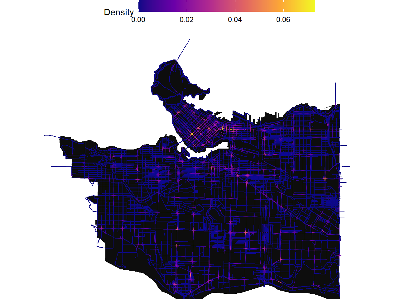
Zooming into downtown:
ggplot() +
  geom_sf(data=study_area,color=NA,fill="gray5")+
  geom_sf(data = collisions_network_kde$network_kde,aes(color=kde_bw_150))+
  scale_color_viridis_c(option = "C",direction = 1,name="Density") +
  theme_void()+
  theme(panel.background= element_rect(fill = NA,color=NA),
        legend.position = "top",
        legend.title.align = 0,
        legend.key.size = unit(1, 'cm'), #change legend key size
        legend.key.height = unit(0.5, 'cm'), #change legend key height
        legend.key.width = unit(1.5, 'cm'))+
  coord_sf(xlim = c(491321.39853389-1000,491321.39853389+1000),
           ylim = c(5459015.689874-1000,5459015.689874+1000))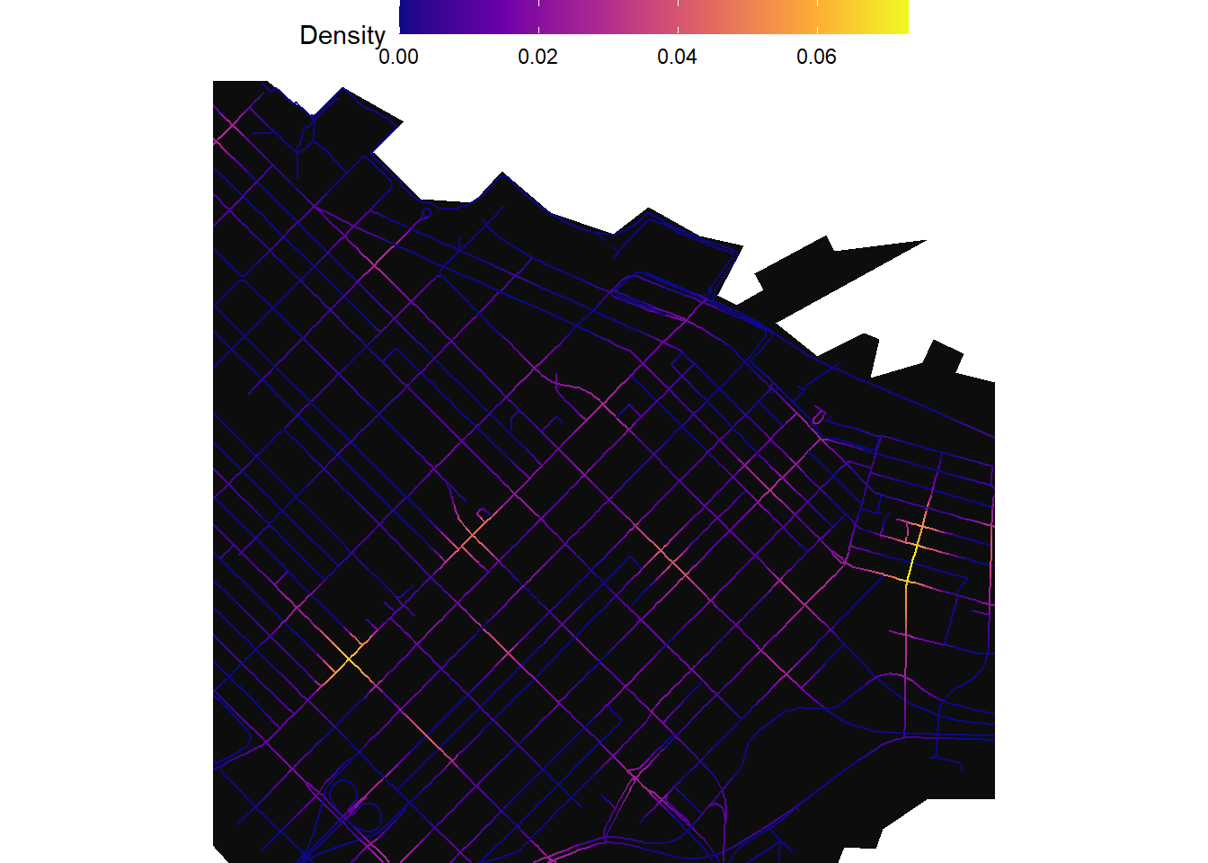
That’s the network KDE function as it is for now. Some challenges going forward are computation time for higher resolution pixels and implementing different kernels other than quartic.
Reproducibility receipt
## [1] "2021-01-22 15:18:01 PST"## Local: main D:/GitHub/website-mbc
## Remote: main @ origin (https://github.com/mbcalles/website-mbc.git)
## Head: [89d6e85] 2020-10-27: Delete 092g01_e.dem## R version 4.0.3 (2020-10-10)
## Platform: x86_64-w64-mingw32/x64 (64-bit)
## Running under: Windows 10 x64 (build 19041)
##
## Matrix products: default
##
## locale:
## [1] LC_COLLATE=English_Canada.1252 LC_CTYPE=English_Canada.1252
## [3] LC_MONETARY=English_Canada.1252 LC_NUMERIC=C
## [5] LC_TIME=English_Canada.1252
##
## attached base packages:
## [1] parallel stats graphics grDevices utils datasets methods
## [8] base
##
## other attached packages:
## [1] doParallel_1.0.16 iterators_1.0.13 foreach_1.5.1 stringr_1.4.0
## [5] ggplot2_3.3.2 sf_0.9-6 dplyr_1.0.2 osmdata_0.1.3
## [9] cancensus_0.3.2 stplanr_0.7.2 igraph_1.2.6 tidygraph_1.2.0
##
## loaded via a namespace (and not attached):
## [1] Rcpp_1.0.5 lubridate_1.7.9.2 lattice_0.20-41 tidyr_1.1.2
## [5] class_7.3-17 digest_0.6.27 R6_2.5.0 evaluate_0.14
## [9] e1071_1.7-4 httr_1.4.2 blogdown_0.21 pillar_1.4.7
## [13] flock_0.7 rlang_0.4.9 curl_4.3 geosphere_1.5-10
## [17] raster_3.3-13 rmarkdown_2.6 labeling_0.4.2 bigparallelr_0.2.5
## [21] foreign_0.8-80 munsell_0.5.0 compiler_4.0.3 xfun_0.18
## [25] pkgconfig_2.0.3 rgeos_0.5-5 htmltools_0.5.0 tidyselect_1.1.0
## [29] tibble_3.0.4 bigstatsr_1.2.3 bookdown_0.21 codetools_0.2-16
## [33] viridisLite_0.3.0 crayon_1.3.4 withr_2.3.0 grid_4.0.3
## [37] jsonlite_1.7.2 lwgeom_0.2-5 gtable_0.3.0 lifecycle_0.2.0
## [41] DBI_1.1.0 git2r_0.27.1 magrittr_2.0.1 units_0.6-7
## [45] scales_1.1.1 KernSmooth_2.23-17 stringi_1.5.3 farver_2.0.3
## [49] sp_1.4-4 xml2_1.3.2 ellipsis_0.3.1 generics_0.1.0
## [53] vctrs_0.3.5 cowplot_1.1.0 geojsonsf_2.0.1 tools_4.0.3
## [57] glue_1.4.2 purrr_0.3.4 yaml_2.2.1 colorspace_2.0-0
## [61] bigassertr_0.1.3 maptools_1.0-2 classInt_0.4-3 rvest_0.3.6
## [65] knitr_1.30